Gallery
Car and trailer, December 2024; with Alejandro Bravo-Doddoli

Mathemematica notebook here
AutoPark, March 2019, May 2020; with Damoon Soudbakhsh and the AutoPark team
Cooperative choreography planning for the Reeds-Shepp car (see Wikipedia on the Dubins car):
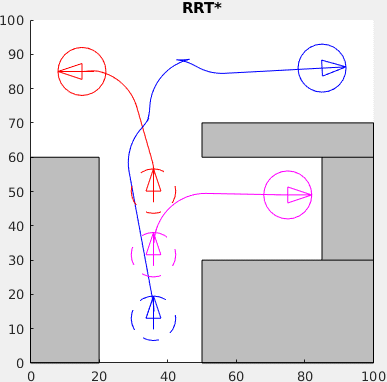

The simultaneous trajectories to the final destinations were computed using the RRT* algorithm.
Here's a demo of RRT* exploring the complement of a square:


Convex Hull, November 2018; with Sara Maloni
A quick Mathematica notebook generating the convex hull in hyperbolic 3-space of a set of points in the plane:
The goal here of the illustration above is to illustrate that the width of the convex hull of a cusp is infinite. Quasicircles generally have finite-width convex hulls, while the converse is false: more complicated non-quasi-circles can have finite width.
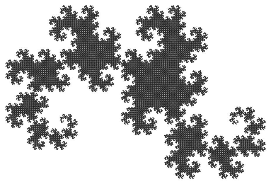
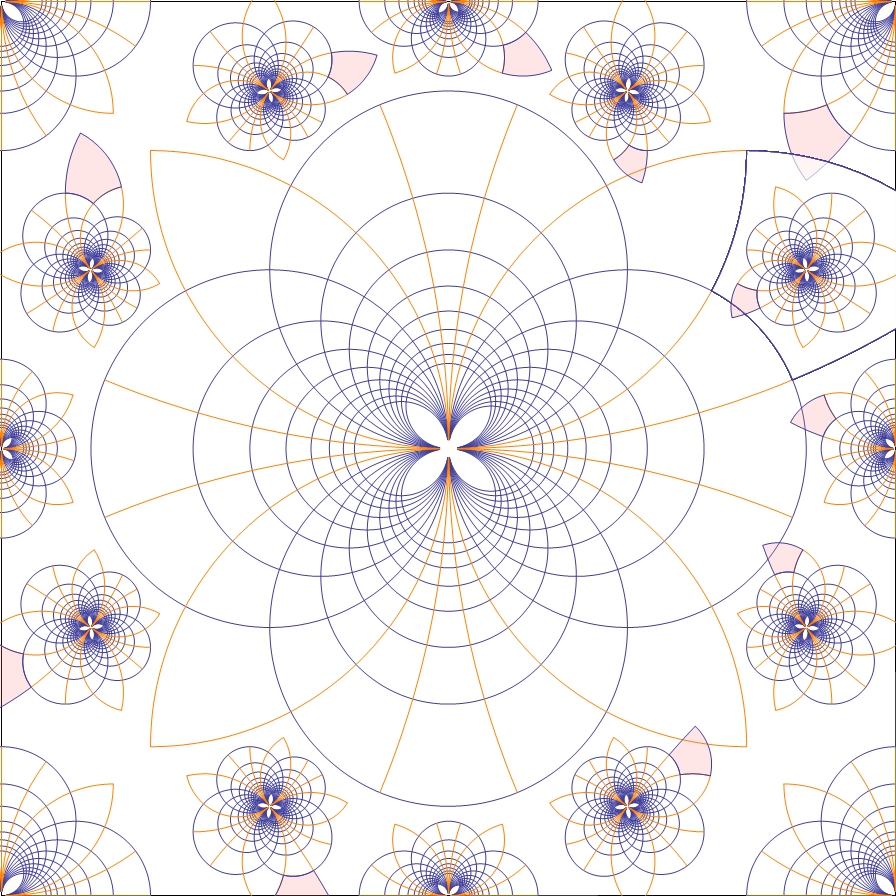
Dragon Curve, April 2018
A quick Mathematica notebook generating the Dragon curve:
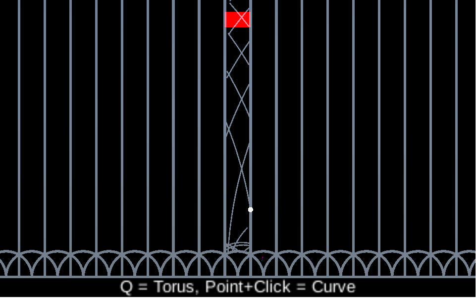
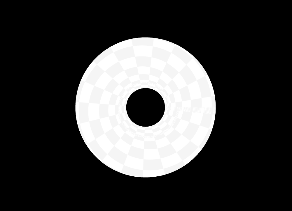
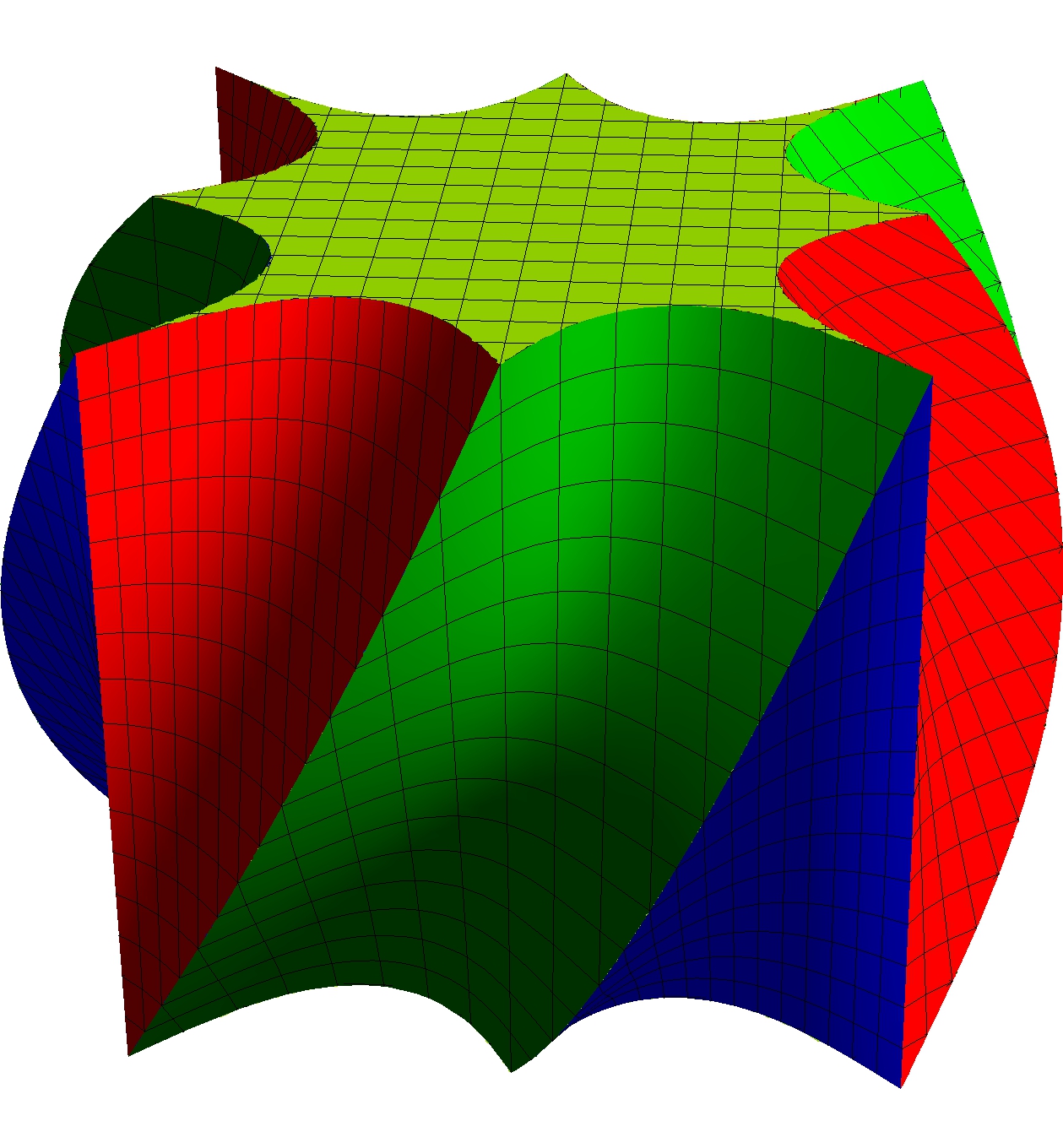
Visualizing SL(2,R)
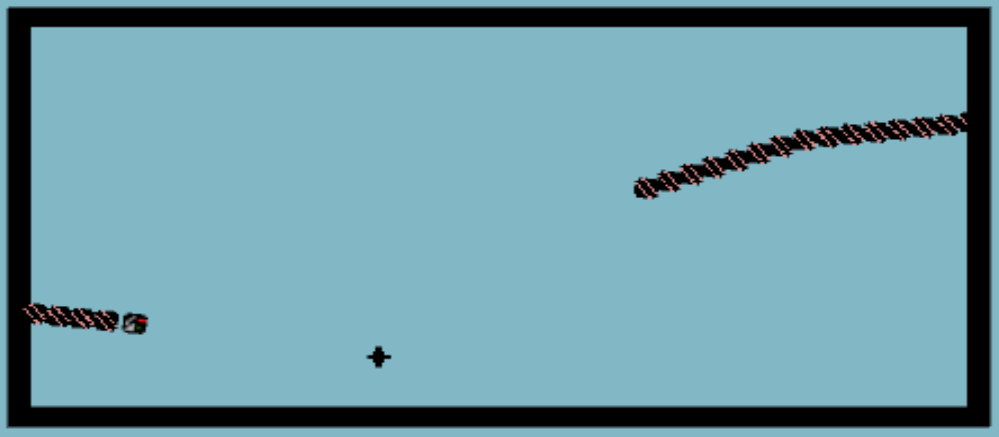
MEGL Project by Joseph Frias, Fall 2017
Click the images for an interactive visualization of geodesic flow on the modular surface SL(2,R)/SL(2,Z). Once in the app, click to shoot the "soccer ball" along a hyperbolic geodesic, and try to hit the red "goal". Notice that the geodesic is normalized using SL(2,Z) symmetry to always stay in the starting tile; and that even though it's hard to hit the goal directly, it's remarkably hard to MISS it if you give the ball time to bounce around (this is due to ergodicity of geodesic flow on the modular surface). Press Q to visualize the location of the soccer ball as a Clifford torus in top view.
Snowballs, March 2017
A 3D variation on the von Koch snowflake. Download the Mathematica notebook or Notebook and images.
Five iterations for the 3-snowball (click for higher resolution):

Two more views of Step 3, showing the "stairway" and the larger square:

Four iterations of the 5-snowball:

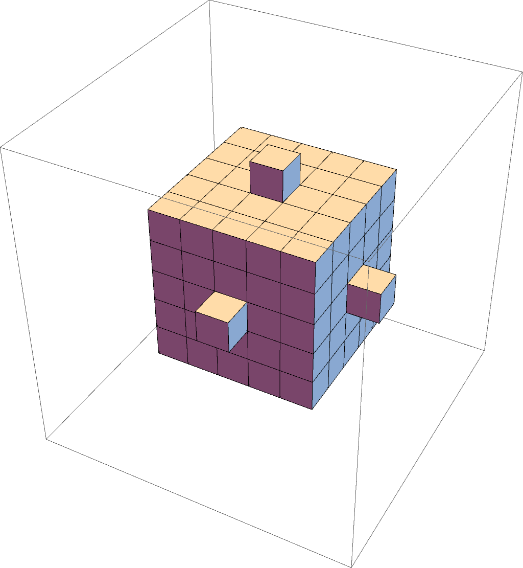
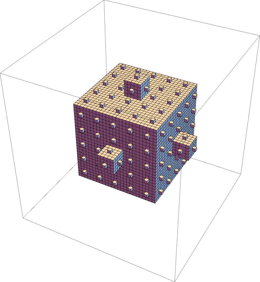

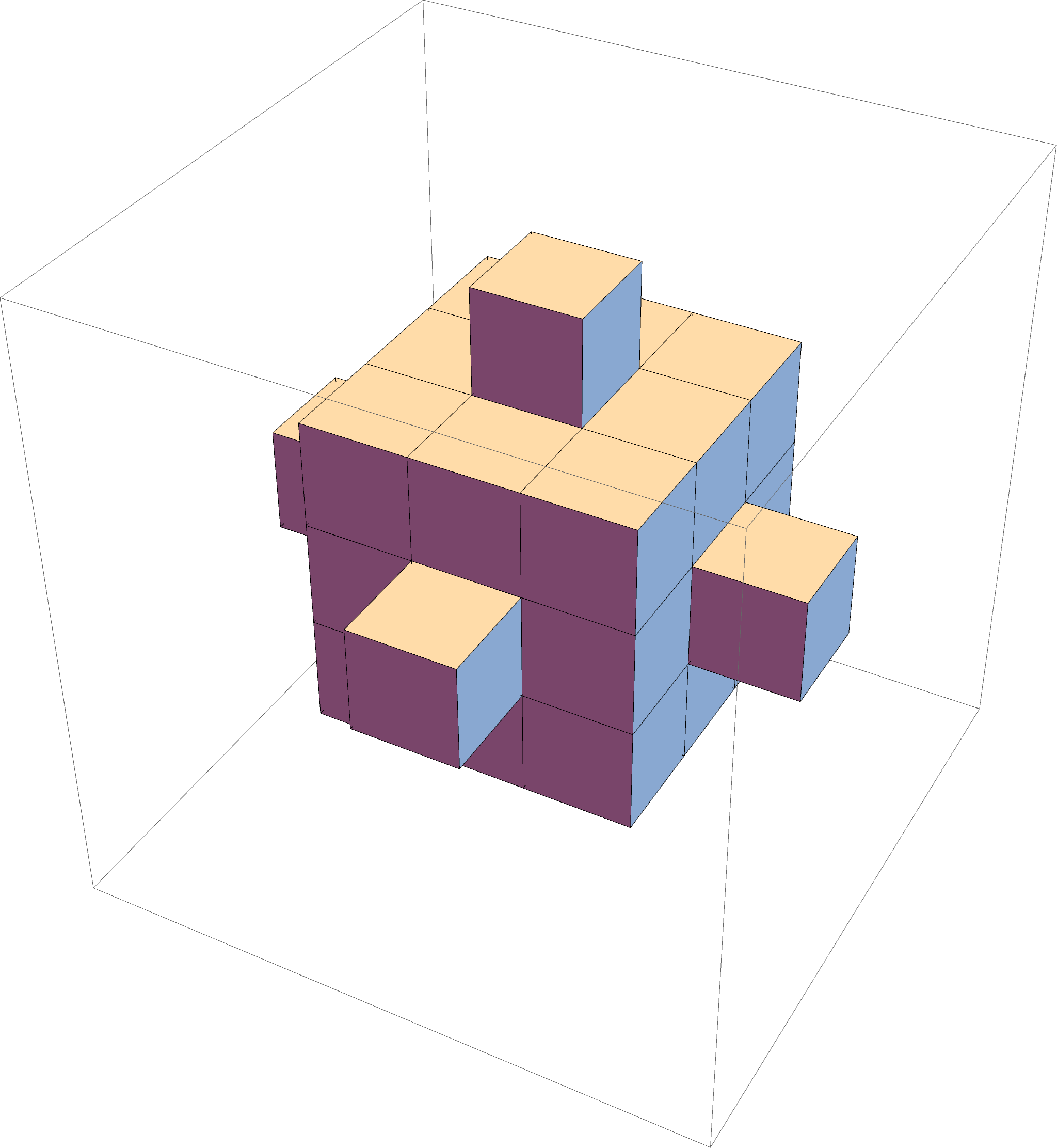
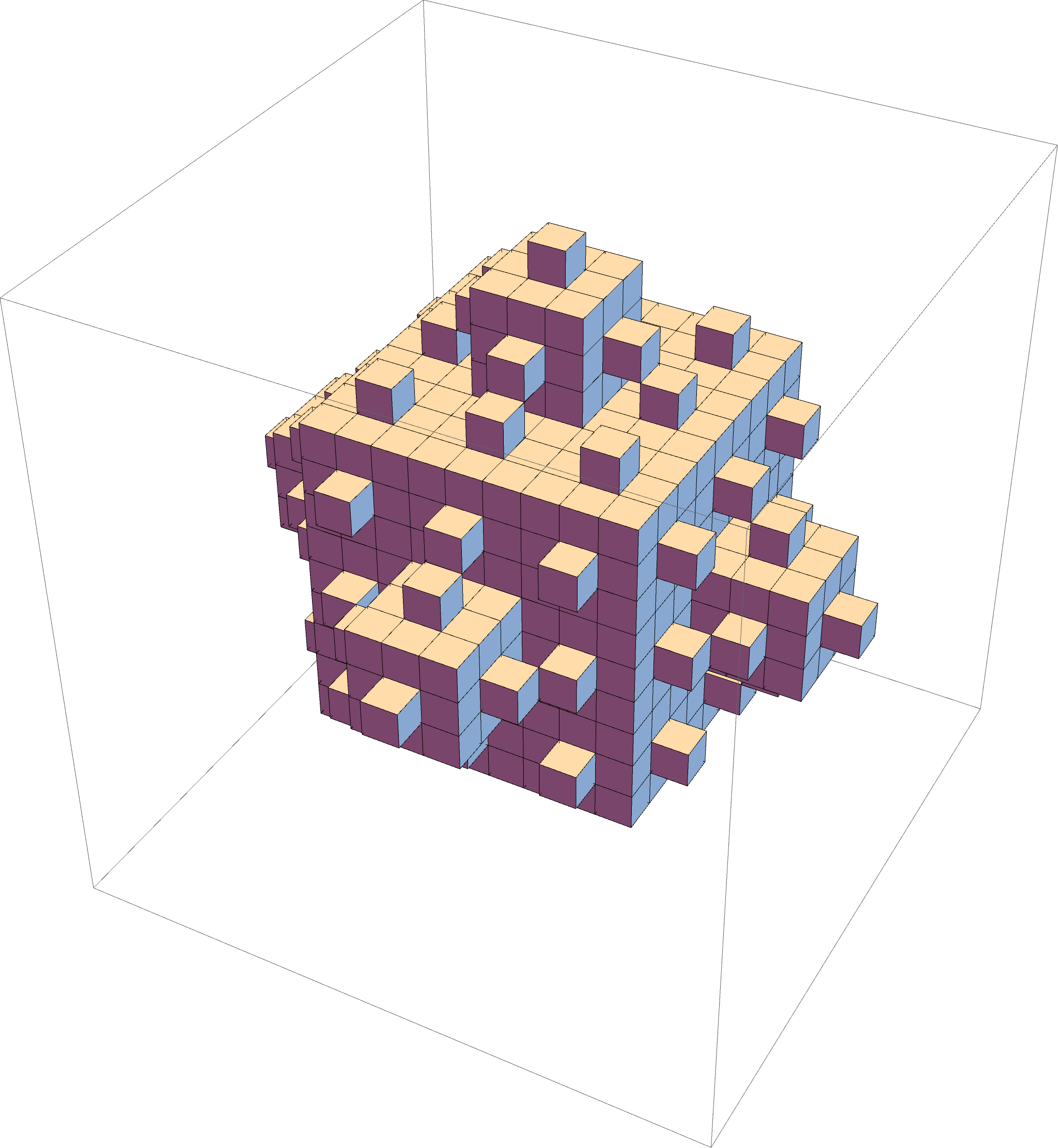
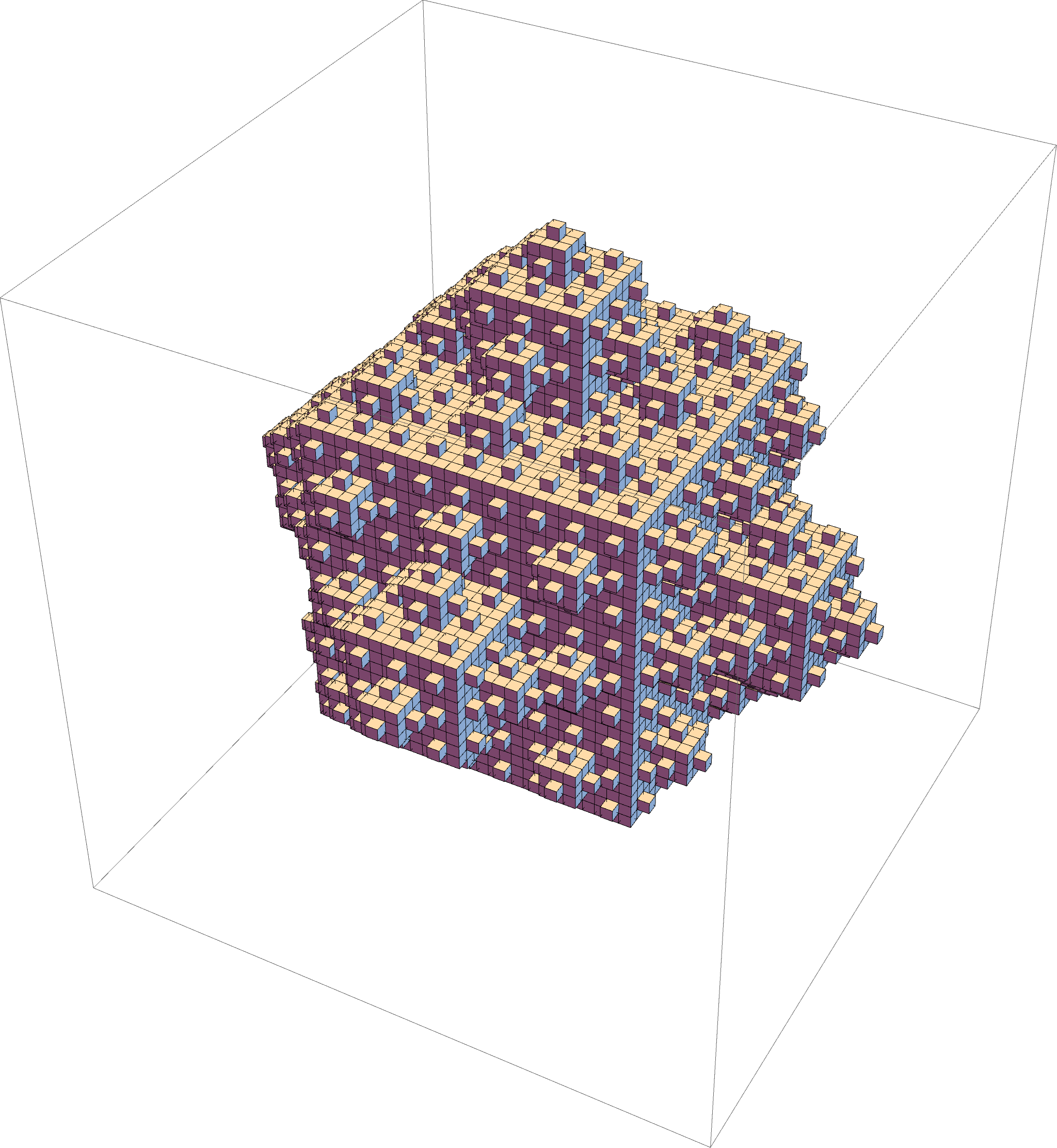
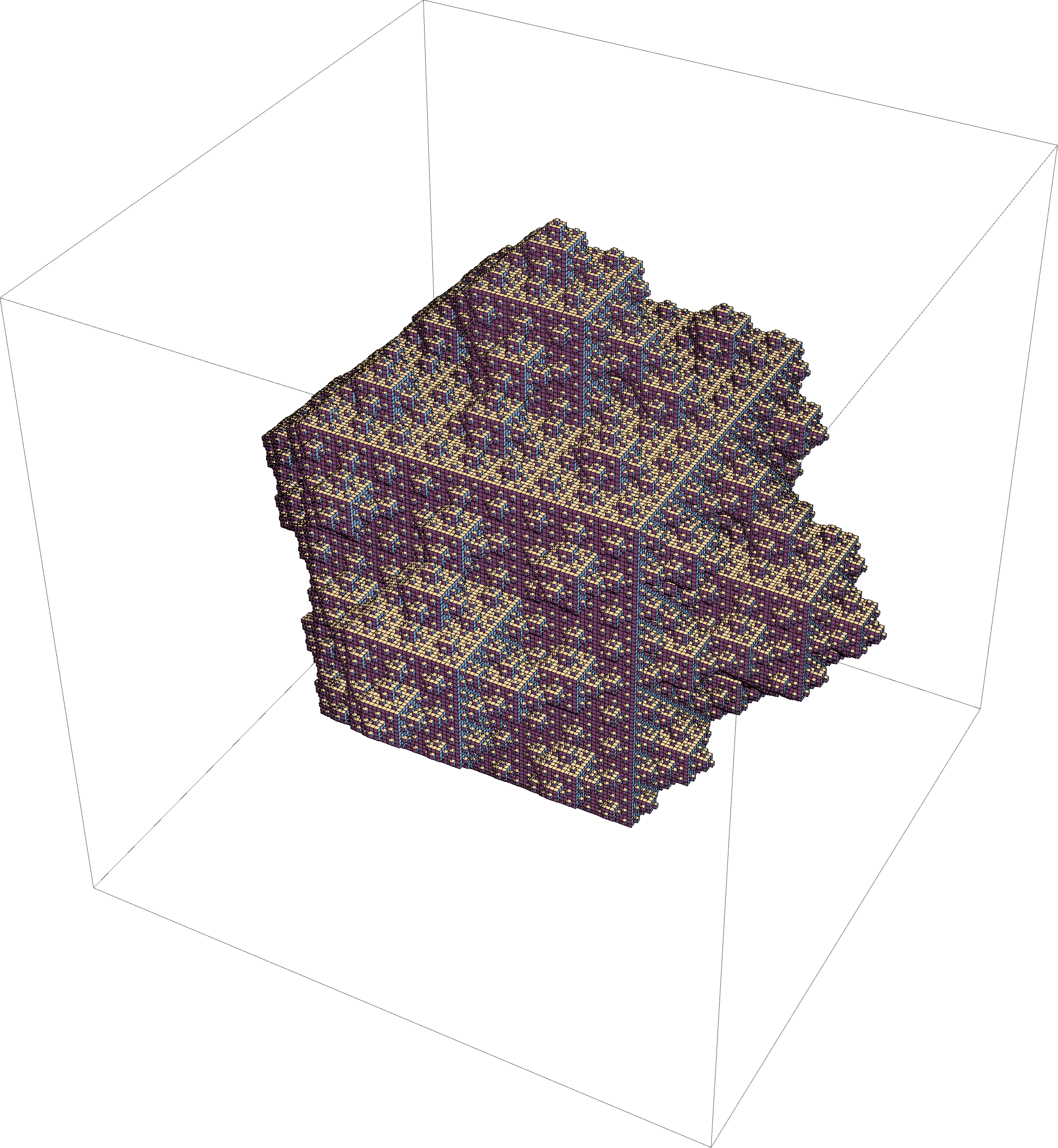
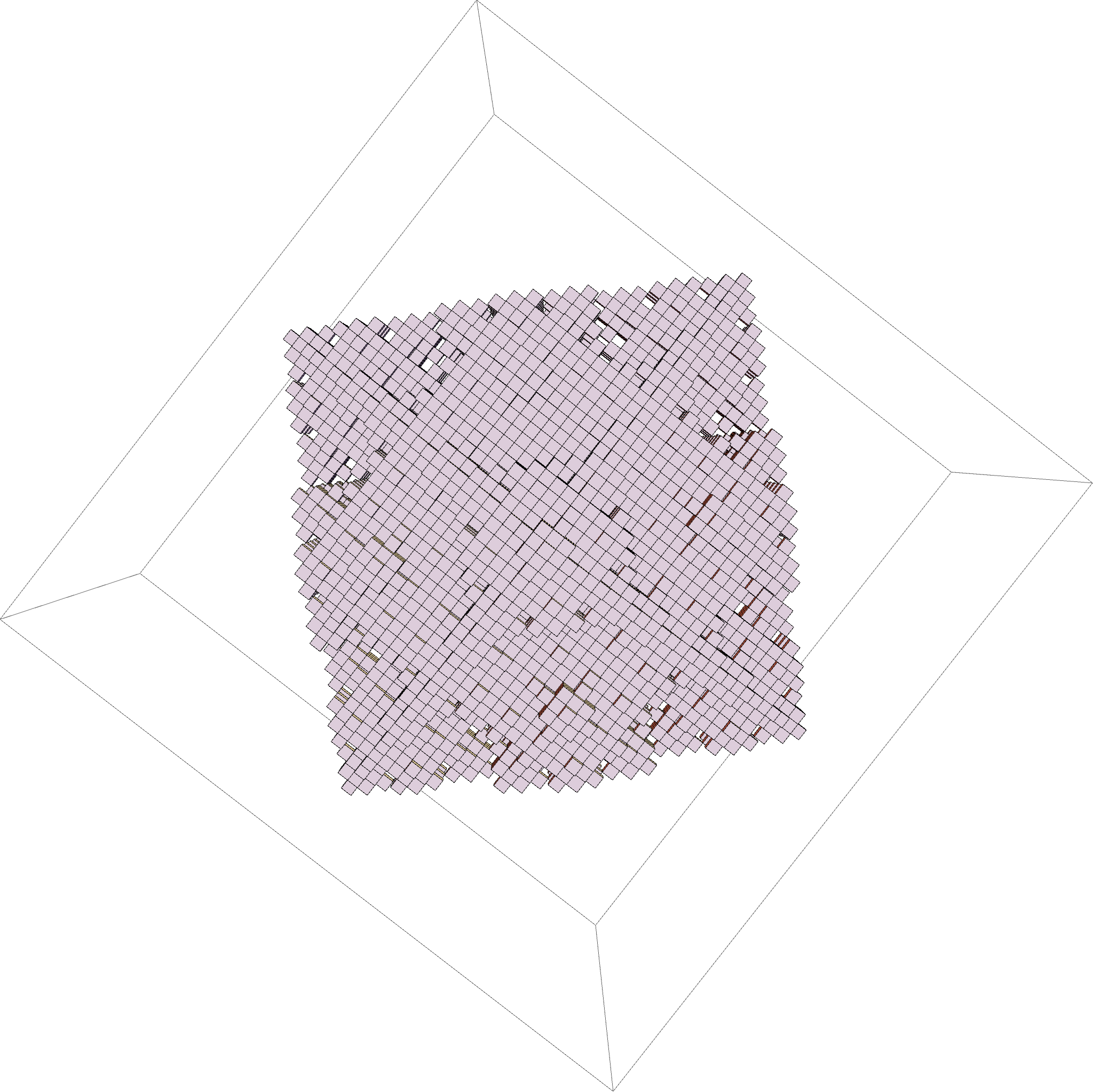
Hakobyan-Herron Maze
In the paper Quasiconvexity in the Heisenberg group David Herron, Jeremy Tyson, and I generalized the work of Hrant Hakobyan and David Herron to the Heisenberg setting. The previous work showed a maze in n-dimensional space whose area (Hausdorff n-1-measure) is zero can always be circumvented with bounded multiplicative cost. As soon as the area zero requirement is violated, even by a fractal maze, this property disappears: there is a maze that is totally disconnected that is infinitely hard to circumvent. The example was built by taking the pre-maze in the illustration below, and inductively replacing each block with copies of the same maze. The limiting fractal object still has dimension $n-1$, is totally disconnected, but has positive "surface area" and a non-quasiconvex complement. My work with Herron and Tyson generalized both results to the Heisenberg group, with n-1 replaced with Q-1.
Snakes in the plane (2015)
REU project by Vaqaas Aslam and Rishee Batra
Snakes in the Plane is a variation on the old game of Snake, in which the player navigates a snake around a map trying to eat food. Every time the snake eats, its tail gets longer - and colliding with either its tail or a wall kills the snake. In our version, the snake can live not only on a simple rectangle but also on such surfaces as torus, Mobius strip, or Klein bottle among others. We hope this game serves as an interesting and informative exploration of what motion on these types of surfaces looks like, and we also hope you enjoy playing it!
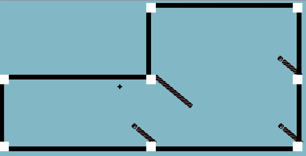
Download the game for: PC or Mac.
Complex and Heisenberg continued fractions (2013-2014)
Continued fractions are a way of writing numbers as infinite fractions. For example, e=2+1/(1+1/(2+1/(1+...))), which is also written
as e=[2; 1,2,1,1,4,1,1,6,...]. To obtain these digits, you take the integer part of the number getting the fracitonal part, and then divide
1 by the fractional part --- and then keep going forever to get all the digits. The process is captured by the Gauss map.
The Gauss map is relatively straightforward for real numbers, but gets messy for complex numbers. In the complex case,
one starts with some region like the unit square centered at the origin and applies the same procedure as before. Different parts of the
square have different starting digits.

Most of these regions still look like distorted squares --- except for the red one that wants to stick out of the square, and the rest of the
regions (not drawn in) along the edge of the square. Things get even worse if we specify the first two digits:
Suppose you start with a random point in the square and apply the invert-truncate "Gauss map" over and over. It is known that for most starting points, you end up visiting every region of the square, but not equally often. Strangely enough, the frequency with which you visit different parts of the square is the same for pretty much any point.
What is NOT known is what happens if you move the square a bit. It appears that the Gauss map still behaves similarly.
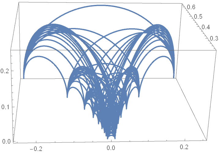
Here are the results of some experiments with moving the square. Here, for each frame of the video I picked points randomly
and applied the Gauss map to them to see how often they visited different parts of the square. It is known that the first frame here
is correct, but no one knows what the other frames ACTUALLY look like.

We can play the same game in hyperbolic space. There, instead of the square we use the following region:
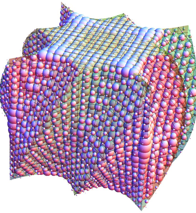
The corresponding invariant density is hard to show. Below, we (me and Joseph Vandehey) place spheres at each point.
The bigger the sphere, the more often the Gauss map visited that part of the "square".